The Detectability Limitation of Community(EN)

27 Jul 2022

This is a note mainly about the paper in 2011：Asymptotic analysis of SBM. And also other paper corresponding with this topic: Cristo Moore,

There exists some concept: Belief Propagation, Bethe free energy, Phase transition, etc. Making note here to clear my mind.

SBM Definition & Question

\(q\) - the number of the groups.

\(n_a\) - the expected fraction of node in group \(a\).

\(N\) - the number of nodes.

\(p_{ab}\) - \(q\times q\) affinity matrix, the probability of an edge between group \(a\) and group \(b\)

\(q_i\) - the group label of node i.

\(N_a = N\times n_a\) - the number of nodes in group \(a\).

\(c_{ab} = N\times p_{ab}\) - the rescaled affinity matrix.

\(M_{ab}=p_{ab}N_aN_b\) - the average number of edges between group a and b.

\(M_{aa}=p_{aa}N_a(N_a-1)\) - the average number of edges in group a.

\(M\) - the number of edges.

Average degree \(c\) for \(N\to \infty\)

Directed Graph For directed graph, average degree means average out degree. Each edge contribute 1 out-degree. So for directed graph, \(c=\frac{edge\ number}{node\ number}\):
\[\begin{aligned}c&=lim_{N\to \infty}\frac{\sum_{a \neq b}p_{ab}Nn_aNn_b+\sum_{a==b}p_{aa}Nn_a(Nn_a-1)}{N}\\&=\sum_{a \neq b}c_{ab}n_an_b+\sum_{a==b}c_{aa}n_an_a\\&=\sum_{a,b}c_{ab}n_an_b\end{aligned}\]
Undirected Graph

For undirected graph, \(c=\frac{2*edge\ number}{node\ number}\):
\[\begin{aligned}c&=lim_{N\to\infty}\frac{2\sum_{a<b}p_{ab}Nn_aNn_b+2\sum_{a==b}p_{aa}Nn_a(Nn_a-1)/2}{N}\\&=2\sum_{a<b}c_{ab}n_an_b+\sum_{a}c_{aa}n_a^2\end{aligned}\]
❓ This result is twice of the result in the paper, see equation(2) in paper. TODO

Question

Base on G，What is the most possible SBM’s parameter \(\begin{aligned}\theta=\left\lbrace q,\left\lbrace n_a\right\rbrace ,\left\lbrace p_{ab}\right\rbrace \right\rbrace \end{aligned}\): parameter learning
Base on G and parameter \(\theta\), What is the most possible group label \(q_i\): inferring the group assignment

For second question, we can first consider a simple question: how to quantify the good of \(\left\lbrace q_i\right\rbrace\). Assume true label is \(\left\lbrace t_i\right\rbrace\), a direct idea is to caculate the number of \(\left\lbrace q_i\right\rbrace\) same with \(\left\lbrace t_i\right\rbrace\).Because different permutation of \(\left\lbrace q_i\right\rbrace\) will change this number, we can select the best result over all permutaion, note as:

\[agreement:A(\left\lbrace t_i\right\rbrace ,\left\lbrace q_i\right\rbrace )=max_\pi\frac{\sum_i\delta_{t_i, \pi(q_i)}}{N}\]

Of which, \(\pi\) is different permutaion for node label.

A simple way to guess node label is that let every node’s label be the label of largest group. Base on the agreement of this way, we can define a kind of normalized agreement, called overlap:

\[overlap:Q(\left\lbrace t_i\right\rbrace ,\left\lbrace q_i\right\rbrace )=max_\pi\frac{\frac{1}{N}\sum_i\delta_{t_i, \pi(q_i)}-max_an_a}{1-max_an_a}\]

\(overlap\) range 0 ~ 1, the bigger the better. When \(\left\lbrace q_i\right\rbrace\) is the same with \(\left\lbrace t_i\right\rbrace\), \(overlap = 1\).

Bayesian Inference & Statistical Physics

Bayesian for inferring the group assignment

Assume that we have solved parameter learning, and get parameter \(\theta\). After given \(\theta\), the probability of generating graph \(G\)(the adjacent matrix is A) and with node label \(\left\lbrace q_i\right\rbrace\) is:

\[\begin{aligned}P(\left\lbrace q_i\right\rbrace ,G|\theta)=\prod_{i\neq j}[p_{q_iq_j}^{A_{ij}}(1-p_{q_iq_j})^{1-A_{ij}}]\prod_in_{q_i}\end{aligned}\tag{2.1.1}\]

In most case, we know the graph G. So what we really want to know is \(P(\left\lbrace q_i\right\rbrace \vert G, \theta)\). According to the Bayesian formula:

\[\begin{aligned}P(\left\lbrace q_i\right\rbrace |G, \theta)&=\frac{P(\left\lbrace q_i\right\rbrace ,G,\theta)}{\sum_{t_i}P(\left\lbrace t_i\right\rbrace ,G,\theta)}\\&=\frac{P(\left\lbrace q_i\right\rbrace ,G|\theta)P(\theta)}{\sum_{t_i}P(\left\lbrace t_i\right\rbrace ,G|\theta)P(\theta)}\\P(\left\lbrace q_i\right\rbrace |G, \theta)&=\frac{P(\left\lbrace q_i\right\rbrace ,G|\theta)}{\sum_{t_i}P(\left\lbrace t_i\right\rbrace ,G|\theta)}\end{aligned}\tag{2.1.2}\]

So substitute (2.1.1) into (2.1.2), we can get formula of \(P(\left\lbrace q_i\right\rbrace \vert G, \theta)\).

Here I clear a confusing point for me. It confuse me that if conditional probability combined with joint probability, such as \(P(A\mid B,C)\). Should it be understood as 1) the conditional probability of A given B,C, or 2) the joint probability of conditional probability of A given B, and the C?

Actually former is right. The condition probability should be priority:
\[\begin{aligned}P(A|B,C)&=\frac{P(A,B,C)}{P(B, C)}\\&=\frac{P(A,B|C)P(C)}{P(B|C)P(C)}=\frac{P(A,B|C)}{P(B|C)}\\&=\frac{P(A,C|B)P(B)}{P(C|B)P(B)}=\frac{P(A,C|B)}{P(C|B)}\end{aligned}\]
It seems like 2) is right, but it should be derived from 1).

Boltzmann distribution

The right part of (2.1.2) is similar with Boltzmann Distribution in Statistical Physics. Assume that a system consists of \(N\) particles, the state of particle \(i\) is \(x_i\). When the system is in state \(\left\lbrace x\right\rbrace\), the energy of the whole system is \(E(\left\lbrace x\right\rbrace )\). And then the boltzmann distribution of the system state \(\left\lbrace x\right\rbrace\) is:

\[p(\left\lbrace x\right\rbrace )=\frac{e^{-\beta E(\left\lbrace x\right\rbrace )}}{Z(\beta)}, where\ Z(\beta)=\sum_{\left\lbrace x^`\right\rbrace \in S}e^{-\beta E(\left\lbrace x^`\right\rbrace )}\tag{2.2.1}\]

In stable condition, the relationship of this ditribution and system energy is:

\[P(\left\lbrace x\right\rbrace )\propto e^{-\beta H(\left\lbrace x\right\rbrace )}\]

Here \(H(\left\lbrace x\right\rbrace )\) is similar to \(E(\left\lbrace x\right\rbrace )\), called Hamiltonian.

Setting \(\beta=1\), \(\left\lbrace q_i\right\rbrace\) in (2.1.2) is the system state. So, the \(H(\left\lbrace q_i\right\rbrace )\) of the system in state \(\left\lbrace q_i\right\rbrace\) is:

\[\begin{aligned}H(\left\lbrace q_i\right\rbrace )&=-logP(\left\lbrace q_i\right\rbrace , G|\theta)\\&=-\sum_{i\neq j}[A_{ij}log\ p_{q_iq_j}+(1-A_{ij})log(1-p_{q_iq_j})]-\sum_ilog\ n_{q_i}\\&=-\sum_{i\neq j}[A_{ij}log\ \frac{c_{q_iq_j}}{N}+(1-A_{ij})log(1-\frac{c_{q_iq_j}}{N})]-\sum_ilog\ n_{q_i}\\&=-\sum_{i\neq j}[A_{ij}log\ c_{q_iq_j}+(1-A_{ij})log(1-\frac{c_{q_iq_j}}{N})]-\sum_ilog\ n_{q_i}+\sum_{i\neq j}A_{ij}logN\\H(\left\lbrace q_i\right\rbrace )&=-\sum_{i\neq j}[A_{ij}log\ c_{q_iq_j}+(1-A_{ij})log(1-\frac{c_{q_iq_j}}{N})]-\sum_ilog\ n_{q_i}\ (ignore\ MlogN)\end{aligned}\tag{2.2.2}\]

❓Here it ignore the last term, I think it’s ignore the term not related with \(\left\lbrace q_i\right\rbrace\). But in paper, they want the energy extensive, make some attribute proportional with \(N\)TODO.

Then, the Boltzmann Distribution of this system and the partition function is:

\[\begin{aligned}\mu(\left\lbrace q_i\right\rbrace |G,\theta)&=\frac{e^{-H(\left\lbrace q_i\right\rbrace )}}{\sum_{\left\lbrace q_i\right\rbrace }e^{-H(\left\lbrace q_i\right\rbrace )}}\end{aligned}\tag{2.2.3}\] \[Z(G,\theta)=\sum_{\left\lbrace q_i\right\rbrace }e^{-H(\left\lbrace q_i\right\rbrace )}\tag{2.2.4}\]

Bayesian for parameter learning

Last section we assume that we have known \(\theta= \left \lbrace q, \left\lbrace n_a\right\rbrace , \left\lbrace p_{ab}\right\rbrace \right \rbrace\). But normally, we only know graph \(G\), so we need to solve \(P(\theta\mid G)\). From Bayesian formula:

\[P(\theta|G)=\frac{P(\theta)}{P(G)}P(G|\theta)=\frac{P(\theta)}{P(G)}\sum_{\left\lbrace q_i\right\rbrace }P(\left\lbrace q_i\right\rbrace ,G|\theta)\]

\(p(\theta)\) is the prior, \(P(\theta\mid G)\) is the posterior. We make no assumption about distribution of \(\theta\), just uniform. So, maximize posterior can be seen as maximize \(\sum_{\left\lbrace q_i\right\rbrace }P(\left\lbrace q_i\right\rbrace ,G\vert \theta)\). From (2.2.2) and (2.2.4), this is just maximize partition function \(Z(G,\theta)\). It’s also equal to minimize free energy density:

\[f(G,\theta)=lim_{N\to \infty}\frac{F_N(G,\theta)}{N}=lim_{N\to \infty}\frac{-logZ(G,\theta)}{N}\]

But what is free energy? what is free energy density?

Free Energy

Thermodynamic potentials

Free energy \(F(\beta)\) is an important thermodynamic potentials. Consider a system represented by (2.2.1):

\[p(\left\lbrace x\right\rbrace )=\mu_\beta(\left\lbrace x\right\rbrace )=\frac{e^{-\beta E(\left\lbrace x\right\rbrace )}}{Z(\beta)}, where\ Z(\beta)=\sum_{\left\lbrace x^`\right\rbrace \in S}e^{-\beta E(\left\lbrace x^`\right\rbrace )}\]

\(Z(\beta)\) is partition function, \(\beta\) is the reciprocal of temperature T: \(\beta=\frac{1}{T}\). Free energy \(F(\beta)\) is defined with logrithm of \(Z(\beta)\) multiply negative temperature.

\[F(\beta)=-\frac{1}{\beta}logZ(\beta)\tag{2.4.1}\]

Other 2 important thermodynamic potentials is internal energy \(U(\beta)\) and canonical entropy \(S(\beta)\):

\[\begin{aligned}U(\beta)=\frac{\partial(\beta F(\beta))}{\partial \beta}\\S(\beta)=\beta^2\frac{\partial F(\beta)}{\partial \beta}\end{aligned}\tag{2.4.2}\]

Further we derive the relationship of \(F(\beta)\), \(U(\beta)\), \(S(\beta)\):

\[\begin{aligned}U(\beta)&=-\frac{\partial log(Z(\beta))}{\partial \beta}=-\frac{Z'(\beta)}{Z(\beta)}\\S(\beta)&=\beta^2\frac{\partial F(\beta)}{\partial \beta}=-\beta^2\frac{\frac{Z'(\beta)}{Z(\beta)}\beta-logZ(\beta)}{\beta^2}=logZ(\beta)-\beta\frac{Z'(\beta)}{Z(\beta)}\\F(\beta)&=U(\beta)-\frac{1}{\beta}S(\beta)\end{aligned}\tag{2.4.3}\]

Substitute \(Z(\beta)=\sum_{\left\lbrace x^`\right\rbrace \in S}e^{-\beta E(\left\lbrace x^`\right\rbrace )}\) into \(U(\beta)\), \(S(\beta)\):

\[\begin{aligned}U(\beta)&=\frac{\sum_{\left\lbrace x^`\right\rbrace \in S}E(\left\lbrace x^`\right\rbrace )e^{-\beta E(\left\lbrace x^`\right\rbrace )}}{Z(\beta)}\\&=\sum_{\left\lbrace x^`\right\rbrace \in S}\frac{e^{-\beta E(\left\lbrace x^`\right\rbrace )}}{Z(\beta)}E(\left\lbrace x^`\right\rbrace )\\&=\left \langle E(\left\lbrace x^`\right\rbrace ) \right \rangle\end{aligned}\tag{2.4.4}\] \[\begin{aligned}S(\beta)&=\beta U(\beta)-\beta F(\beta)\\&=\sum_{\left\lbrace x^`\right\rbrace \in S}\mu_\beta({x^`})\beta E(\left\lbrace x^`\right\rbrace )+log\sum_{\left\lbrace x\right\rbrace \in S}e^{-\beta E(\left\lbrace x\right\rbrace )}\\&=\sum_{\left\lbrace x^`\right\rbrace \in S}\mu_\beta({x^`})\beta E(\left\lbrace x^`\right\rbrace )+\sum_{\left\lbrace x^`\right\rbrace \in S}\mu_\beta({x^`})log\sum_{\left\lbrace x\right\rbrace \in S}e^{-\beta E(\left\lbrace x\right\rbrace )}\\&=\sum_{\left\lbrace x^`\right\rbrace \in S}\mu_\beta({x^`})(\beta E(\left\lbrace x^`\right\rbrace )+log\sum_{\left\lbrace x\right\rbrace \in S}e^{-\beta E(\left\lbrace x\right\rbrace )})\\&=\sum_{\left\lbrace x^`\right\rbrace \in S}\mu_\beta({x^`})(-log\ e^{-\beta E(\left\lbrace x^`\right\rbrace )}+log\sum_{\left\lbrace x\right\rbrace \in S}e^{-\beta E(\left\lbrace x\right\rbrace )})\\&=-\sum_{\left\lbrace x^`\right\rbrace \in S}\mu_\beta({x^`})log\ \mu_\beta({x^`})\end{aligned}\tag{2.4.5}\]

We can see that \(U(\beta)\) is the average system energy according to Boltzmann Distribution. And \(S(\beta)\) is the entropy of Boltzmann Distribution.

Thermodynamic limit

The free energy is scaled with system size \(N\). Free energy density is that when \(N\to\infty\), the limitation of free energy for every particles：

\[f(\beta)=lim_{N\to \infty}\frac{F_N(\beta)}{N}\]

Similarly we can defined energy density \(u(\beta)\)和 entropy density \(s(\beta)\).

Ising Model(See Post Later)

Parameter learning

Sec. IIC. TODO

Cavity Method & Belief Propagation

From (2.2.3)：

We known the joint probability distribution of all nodes’ label \(\mu(\left\lbrace q_i\right\rbrace )\). But if we want to know a certain node label’s distribution, that is marginal distribution, we need to know:

\[v_i(q_i)=\sum_{\left\lbrace q_j\right\rbrace _{j\neq i}}\mu(\left\lbrace q_j\right\rbrace _{j\neq i},q_i)\]

To solve the marginal distribution, a classical method is Belief Propagation(BP), which is also called Cavity Method in statistical Physics. In Ising model, the state of every particle depended on its neighbour’s state. If we initial state distribution of all particles, iterate self state distribution from neighbour’s distribution, and finally converge to a distribution as result marginal distribution. So, we can use the similar idea to estimate \(v_i(q_i)\) with BP.

Belief Propagation

Now back to our Community Detection problem. BP algorithm compute node’s marginal probability \(\psi_r^i\) with iterative way, \(\psi_r^i\) means the probabilty of node \(i\) belong to group \(r\). \(\psi_r^i\) is a term of the \(q\) dimensional vector \(\overrightarrow{\psi^i}\):

\[\psi^i=\begin{bmatrix} \psi_1^i& \psi_2^i & ... &\psi_q^i \end{bmatrix}\tag{3.1.1}\]

Naive Bayes(Follow Cristo Moore)

A direct idea is that, neighbour’s marginal will influence self marginal. For example, if node \(i\)’s neighbour \(j\) belong to group \(s\), and the link probability of group \(r\) and \(s\) is \(p_{rs}\). So the edge \((i, j)\) will affect node \(i\)’s marginal \(\psi_r^i\) by \(p_{rs}\psi_s^j\), if node \(j\) belong to group \(s\). Assume node \(i\)’s different neighbour independent with each other, after considering different neighbour of node \(i\), and different group \(s\) for every neighbour node, the relationship between marginal of node \(i\) and marginal of its neighbour nodes is:

\[\psi_r^i\propto\prod_{j:(i,j)\in E}\sum_{s=1}^q\psi_s^jp_{rs}\]

Then iterate it until convergence, get every node’s marginal. However, this idea is so naive, especially the assumption that neighbour nodes is independent with each other. BP change this assumption, node neighbour’s marginal is dependent with each other, but the neighbour’s marginal given by self node is independent with each other. That means neighbour nodes are correlated only through self node.

Belief Propagation(Follow Cristo Moore)

BP define every node \(i\) send message \(\psi^{i\to j}\) to its neighbour \(j\). Just like (3.1.1), this is also a q-dimension vector. \(\psi^{i\to j}_r\) means that if \(i\) didn’t have neighbour \(j\), then what is the marginal probability of node \(i\) belong to group \(r\) estimated only base on \(i\)’s other neighbour. So the core of \(\psi_r^{i\to j}\) is that it means node \(i\)’s marginal distribution. \(^{\to j}\) is only a constraint condition: \(i\) didn’t know neighbout \(j\)。

捕获1

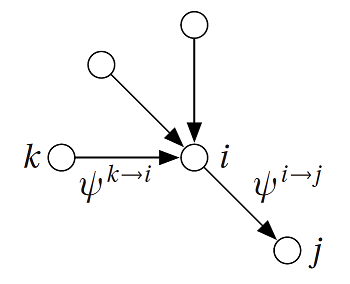
Draw on Naive Bayes’s idea，we can get:

\[\psi_r^{i\to j}\propto\prod_{\begin{aligned}k:(&i,k)\in E\\&k\neq j\end{aligned}}\sum_{s=1}^q\psi_s^{k\to i}p_{rs}\tag{3.1.2}\]

PS: in undirected network, each edge has two message.

BP first initial all messgae in edges, then iterate these message with (3.1.2) until they converge. Finally, compute each node’s marginal distribution base on edge’s message:

\[\psi_r^i\propto\prod_{j:(i,j)\in E}\sum_{s=1}^q\psi_s^{j\to i}p_{rs}\tag{3.1.3}\]

In (3.1.2), \(\psi_r^{i\to j}\) has no correlation with \(\psi_s^{j\to i}\)，this stop self information transfer to self. BP must converge in tree-like graph, but maybe don’t converge in general graph. When graph is sparse, it has locally tree-like part. So the BP will get a good approximation of marginal probability. In this condition, although node’s self marginal distribution will go back to itself after a big circle. But because the circle is too big, self information will be diluted, its effect is not so large.

BP in SBM(Follow Asymptotic)

Assume we have know about Graph G，And the SBM parameter \(\theta=\left \lbrace q, \left\lbrace n_a\right\rbrace , \left\lbrace p_{ab}\right\rbrace \right \rbrace\)。Use BP to finish inferring the group assignment。

Assume node \(i\) can recieve all node’s information, then node \(i\)’s marginal distribution is：

\[\begin{aligned}\psi_{t_i}^{i\to j}&=\frac{1}{Z^{i\to j}}\prod_{k\in \partial i\setminus j}\sum_{t_k}p_{t_it_k}^{A_{ik}}(1-p_{t_it_k})^{1-A_{ik}}\psi_{t_k}^{k\to i}\\&=\frac{1}{Z^{i\to j}}\prod_{k\in \partial i\setminus j}\sum_{t_k}\frac{c_{t_it_k}}{N}^{A_{ik}}(1-\frac{c_{t_it_k}}{N})^{1-A_{ik}}\psi_{t_k}^{k\to i}\\&=\frac{1}{Z^{i\to j}}\prod_{k\in \partial i\setminus j}\frac{1}{N^{A_{ik}}}\sum_{t_k}c_{t_it_k}^{A_{ik}}(1-\frac{c_{t_it_k}}{N})^{1-A_{ik}}\psi_{t_k}^{k\to i}\\&=\frac{1}{Z^{i\to j}}\frac{1}{N^{d_i-1}}\prod_{k\in \partial i\setminus j}\sum_{t_k}c_{t_it_k}^{A_{ik}}(1-\frac{c_{t_it_k}}{N})^{1-A_{ik}}\psi_{t_k}^{k\to i},\ d_i:the\ degree\ of\ i\end{aligned}\]

Here \(\partial i\) means all neighbours which can transfer message to node \(i\). Because of normalization, we can ignore the entry which don’t have \(t_i\), such as \(\frac{1}{N^{d_i-1}}\). And get:

\[\psi_{t_i}^{i\to j}=\frac{1}{Z^{i\to j}}\prod_{k\in \partial i\setminus j}\sum_{t_k}c_{t_it_k}^{A_{ik}}(1-\frac{c_{t_it_k}}{N})^{1-A_{ik}}\psi_{t_k}^{k\to i}\]

But in paper, it is:

\[\psi_{t_i}^{i\to j}=\frac{1}{Z^{i\to j}}n_{t_i}\prod_{k\in \partial i\setminus j}\sum_{t_k}c_{t_it_k}^{A_{ik}}(1-\frac{c_{t_it_k}}{N})^{1-A_{ik}}\psi_{t_k}^{k\to i}\tag{3.1.4}\]

It has an additional \(n_{t_i}\), it is the prior.

And then From (3.1.4)，we can get the marginal probability is：

\[v_i(t_i)=\psi_{t_i}^i=\frac{1}{Z^{i}}n_{t_i}\prod_{k\in \partial i}\sum_{t_k}c_{t_it_k}^{A_{ik}}(1-\frac{c_{t_it_k}}{N})^{1-A_{ik}}\psi_{t_k}^{k\to i}\tag{3.1.5}\]

But this will update message in all edges, the time complexity is high \(O(N^2)\). But, Consider \(N\to \infty\), the information \(i\) send to non-neighbour \(j\) is the same. Assume \((i,j)\notin E\), Here \(\partial i\) means \(i\) real neighbour (has edge connection):

\[\begin{aligned}\psi_{t_i}^{i\to j}&=\frac{1}{Z^{i\to j}}n_{t_i}[\prod_{k\notin \partial i \setminus j}\sum_{t_k}c_{t_it_k}^{A_{ik}}(1-\frac{c_{t_it_k}}{N})^{1-A_{ik}}\psi_{t_k}^{k\to i}][\prod_{k\in \partial i}\sum_{t_k}c_{t_it_k}^{A_{ik}}(1-\frac{c_{t_it_k}}{N})^{1-A_{ik}}\psi_{t_k}^{k\to i}]\\&=\frac{1}{Z^{i\to j}}n_{t_i}[\prod_{k\notin \partial i \setminus j}\sum_{t_k}(1-\frac{c_{t_it_k}}{N})\psi_{t_k}^{k\to i}][\prod_{k\in \partial i}\sum_{t_k}c_{t_it_k}^{A_{ik}}\psi_{t_k}^{k\to i}]\\&=\frac{1}{Z^{i\to j}}n_{t_i}[\prod_{k\notin \partial i \setminus j}1-\frac{1}{N}\sum_{t_k}c_{t_it_k}\psi_{t_k}^{k\to i}][\prod_{k\in \partial i}\sum_{t_k}c_{t_it_k}\psi_{t_k}^{k\to i}]\\&\overset{N\to \infty}{=}\frac{1}{Z^{i\to j}}n_{t_i}[\prod_{k\in \partial i}\sum_{t_k}c_{t_it_k}^{A_{ik}}\psi_{t_k}^{k\to i}]\\&=\psi_{t_i}^i\end{aligned}\]

In this equation, From 2nd line to 3rd line it use \(\sum_{t_k}\psi_{t_k}^{k\to i}=1\).

From 3rd line to 4th line the middle term turn to 1：when \(N\to \infty\)，\(\sum_{t_k}c_{t_it_k}\psi_{t_k}^{k\to i}\) is a constant with comparison with \(N\)，note it as \(C\)。The number of terms to be multiplied together is approximated by \(N\). So the middle term is approximated by \(lim_{N\to \infty}(1-\frac{C}{N})^N=1\).

The message \(i\) send to \(j\)：

\[\begin{aligned}\psi_{t_i}^{i\to j}&=\frac{1}{Z^{i\to j}}n_{t_i}[\prod_{k\notin \partial i }\sum_{t_k}c_{t_it_k}^{A_{ik}}(1-\frac{c_{t_it_k}}{N})^{1-A_{ik}}\psi_{t_k}^{k\to i}][\prod_{k\in \partial i\setminus j}\sum_{t_k}c_{t_it_k}^{A_{ik}}(1-\frac{c_{t_it_k}}{N})^{1-A_{ik}}\psi_{t_k}^{k\to i}]\\&=\frac{1}{Z^{i\to j}}n_{t_i}[\prod_{k\notin \partial i }1-\frac{1}{N}\sum_{t_k}c_{t_it_k}\psi_{t_k}^{k\to i}][\prod_{k\in \partial i\setminus j}\sum_{t_k}c_{t_it_k}\psi_{t_k}^{k\to i}]\\&=\frac{1}{Z^{i\to j}}n_{t_i}[1-\frac{1}{N}\sum_{k\notin \partial i}\sum_{t_k}c_{t_kt_i}\psi_{t_k}^{k\to i}+O(\frac{1}{N^2})][\prod_{k\in \partial i\setminus j}\sum_{t_k}c_{t_it_k}\psi_{t_k}^{k\to i}]\\&\approx \frac{1}{Z^{i\to j}}n_{t_i}e^{-h_{t_i}}[\prod_{k\in \partial i\setminus j}\sum_{t_k}c_{t_it_k}\psi_{t_k}^{k\to i}],\ h_{t_i}=\frac{1}{N}\sum_{k\notin \partial i}\sum_{t_k}c_{t_kt_i}\psi_{t_k}^{k\to i}\end{aligned}\tag{3.1.6}\]

The last line use Taylor Series \(e^{-x}\approx1-x\). Here \(h_{t_i}\) called external field. But in paper \(h_{t_i}\) is：

\[h_{t_i}=\frac{1}{N}\sum_{k}\sum_{t_k}c_{t_kt_i}\psi_{t_k}^{k}\]

❓ The second difference is \(\psi_{t_k}^k\), We can think when \((i,k)\notin E\)，\(\psi_{t_k}^{k\to i}=\psi_{t_k}^{k}\)。The first difference in first sum over \(k\) or \(k\notin \partial i\), maybe because when \(N\to \infty\), these two have no big difference. But I’m not sure TODO.

So, initial all information, iterate with (3.1.6), calculated the marginal probability:

\[v_i(t_i)=\psi_{t_i}^i=\frac{1}{Z^{i}}n_{t_i}e^{-h_{t_i}}\prod_{j\in \partial i}\sum_{t_j}c_{t_it_j}\psi_{t_j}^{j\to i}\tag{3.1.7}\]

Phase Transition

This section, we understand how to locate Kesten-Stigum thereshold in Community Detection:

\[|c_{in}-c_{out}|>q\sqrt{c}\]

Conside a special condition：An undirected graph generated by SBM，the average degree \(c\) for every group \(a\) is equal：

\[\sum_{d=1}^qc_{ad}n_d=\sum_{d=1}^qc_{bd}n_d=c\tag{4.0.1}\]

PS：\(c_{ad}n_d=Np_{ad}n_d=N_dp_{ad}\)，It means the every number of edge which nodes in group \(a\) connect to nodes in group \(d\)，sum it over all group \(d\)，and we get the average degree of group \(a\)

The model satisfied that called：factorized block model.

Factorized Fixed Point

BP in SBM：(3.1.6) and (3.1.7)，has a fixed point (Called factorized fixed point, note as FFP)：

\[\psi_{t_i}^{i\to j}=n_{t_i}\tag{4.1.1}\]

We can substitute (4.1.1) to (3.1.6) to verify it：

\[\begin{aligned}\psi_{t_i}^{i\to j}&=\frac{1}{Z^{i\to j}}n_{t_i}e^{-h_{t_i}}[\prod_{k\in \partial i\setminus j}\sum_{t_k}c_{t_it_k}\psi_{t_k}^{k\to i}]\\&= \frac{1}{Z^{i\to j}}n_{t_i}e^{-\frac{1}{N}\sum_{k\notin \partial i}\sum_{t_k}c_{t_kt_i}\psi_{t_k}^{k\to i}}[\prod_{k\in \partial i\setminus j}\sum_{t_k}c_{t_it_k}n_{t_k}]\\&=\frac{1}{Z^{i\to j}}n_{t_i}e^{-\frac{1}{N}\sum_{k\notin \partial i}\sum_{t_k}c_{t_kt_i}n_{t_k}}[\prod_{k\in \partial i\setminus j}\sum_{t_k}c_{t_it_k}n_{t_k}]\\&=\frac{1}{Z^{i\to j}}n_{t_i}e^{-\frac{1}{N}\sum_{k\notin \partial i}c}[\prod_{k\in \partial i\setminus j}c]\\&=\frac{n_{t_i}e^{-\frac{1}{N}\sum_{k\notin \partial i}c}\prod_{k\in \partial i\setminus j}c}{\sum_{n_{t_i}}n_{t_i}e^{-\frac{1}{N}\sum_{k\notin \partial i}c}\prod_{k\in \partial i\setminus j}c}\\&=n_{t_i}\end{aligned}\]

Substitute this factorized fixed point into (3.1.7)，we get the marginal distribution：

\[\begin{aligned}\psi_{t_i}^i&=\frac{1}{Z^{i}}n_{t_i}e^{-h_{t_i}}\prod_{j\in \partial i}\sum_{t_j}c_{t_it_j}\psi_{t_j}^{j\to i}\\&=\frac{1}{Z^{i}}n_{t_i}e^{-h_{t_i}}\prod_{j\in \partial i}\sum_{t_j}c_{t_it_j}n_{t_j}\\&=\frac{1}{Z^{i}}n_{t_i}e^{-h_{t_i}}\prod_{j\in \partial i}c\\&=n_{t_i}\end{aligned}\]

As we can see, the distribution of node \(i\) is not related with the node \(i\). If we inferring the group assignment base on this distribution, then the group label of every node is the biggest size group. The overlap of this kind of group assignment is 0.

\[Q(\left\lbrace t_i\right\rbrace ,\left\lbrace q_i\right\rbrace )=max_\pi\frac{\frac{1}{N}\sum_i\delta_{t_i, \pi(q_i)}-max_an_a}{1-max_an_a}=\frac{max_aN_a/N-max_an_a}{1-max_an_a}=0\]

The distribution don’t have any useful information about group assignment. If BP converge to this point, then there is no possible to reveal the real group assignment. Base on that, the paper analysis the detectability-undetectability phase transition point in community detection.

Stability of FFP(Follow Asymptotic)

Consider when we perturbate the marginal distribution of BP algorithm, what happen in factorized fixed point?

In a sparse network, it is local tree-like. So, consider a d-level tree and perturbate the marginal distribution in the leaf node when BP come to factorized fixed point:

\[\psi_t^k=n_t + \epsilon_t^k\tag{4.2.1}\]

Then we study the influence of root node when we perturbate all \(c^d\) leaf node. Assume the influence of each leaf node is independent with each other, consider a path \(d,d-1,d-2,...,i+1,i,...,1,0\). We define a transition matrix.：

\[\begin{aligned}T_i^{ab}&=\frac{\partial\psi_a^i}{\partial\psi_b^{i+1}}|_{\psi_t=n_t}\\&=(\frac{\psi_a^ic_{ab}}{\sum_rc_{ar}\psi_r^{i+1}}-\psi_a^i\sum_s\frac{\psi_s^ic_{sb}}{\sum_rc_{ar}\psi_r^{i+1}})|_{\psi_t=n_t}\end{aligned}\tag{4.2.2}\]

for simplicity, I use these symbol \(l, j\) to substitute \(i+1\), \(i-1\), etc.

Actually, the perturbation is propagated through the system through the messages, not directly the marginals themselves. The original paper Asymptotic analysis of SBM also say that this T is derived from BP message passing equation (26). So the real \(T\) should be like this:
\[T_{ab}^i=\frac{\partial \psi_a^{i\to j}}{\partial\psi_b^{l\to i}}, here\ l\ is\ i+1\]
And another point, when network in FFP and satisfy the condition that every group \(a\) has the same degree \(c\). \(\psi^i\) is equal to \(\psi^{i\to j}\), as last section say. So the notation of paper also make sense!

After understand this, we can derive equation (4.2.2):
\[\begin{aligned}\psi_a^{i\to j}&=\frac{1}{Z^{i\to j}}n_ae^{-h_a}\prod_{k\in\partial i/j}\sum_{t_k}c_{t_ka}\psi_{t_k}^{k\to i},\ h_a=\frac{1}{N}\sum_k\sum_{t_k}c_{t_ka}\psi_{t_k}^k\\&=\frac{1}{Z^{i\to j}}n_ae^{-h_a}\sum_{t_l}c_{t_la}\psi_{t_l}^{l\to i},\ only\ node\ l\ in\ \partial i/j\\ln\psi_a^{i\to j}&=ln(n_a)-h_a+ln\sum_{t_l}c_{t_la}\psi_{t_l}^{l\to i} - ln\sum_rn_re^{-h_r}\sum_{t_l}c_{t_lr}\psi_{t_l}^{l\to i},\\&\ Then\ find\ derivative\ by\ \psi_b^{l\to i}\ both\ side\\\frac{\partial \psi_a^{i\to j}}{\partial\psi_b^{l\to i}}\frac{1}{\psi_a^{i\to j}}&=0-0+\frac{c_{ba}}{\sum_{t_l}c_{t_la}\psi_{t_l}^{l\to i}}-\frac{\sum_rn_re^{-h_r}c_{br}}{Z^{i\to j}}\\&=\frac{c_{ba}}{\sum_{t_l}c_{t_la}\psi_{t_l}^{l\to i}}-\frac{\sum_rn_re^{-h_r}c_{br}}{Z^{i\to j}}\frac{\sum_{t_l}c_{t_lr}\psi_{t_l}^{l\to i}}{\sum_{t_l}c_{t_lr}\psi_{t_l}^{l\to i}}\\&=\frac{c_{ba}}{\sum_{t_l}c_{t_la}\psi_{t_l}^{l\to i}}-\sum_r\frac{n_re^{-h_r}\sum_{t_l}c_{t_lr}\psi_{t_l}^{l\to i}}{Z^{i\to j}}\frac{c_{br}}{\sum_{t_l}c_{t_lr}\psi_{t_l}^{l\to i}}\\&=\frac{c_{ba}}{\sum_{t_l}c_{t_la}\psi_{t_l}^{l\to i}}-\sum_r\frac{\psi_r^{i\to j}c_{br}}{\sum_sc_{sr}\psi_s^{l\to i}} \end{aligned}\]
Only a little difference with eqn (4.2.2), the denominator of last term. But it’s has no influence for the following derivation.

From equation (4.2.2), and the assumption about average degree \(c\) (4.0.1)：

\[\begin{aligned}T_i^{ab}&=\frac{n_ac_{ab}}{\sum_rc_{ar}n_r}-n_a\sum_s\frac{n_sc_{sb}}{\sum_rc_{ar}n_r}\\&=\frac{n_ac_{ab}}{c}-n_a\frac{c}{c}\\&=n_a(\frac{c_{ab}}{c}-1)\end{aligned}\tag{4.2.3}\]

Then we get transition matrix. We also can calculate the relationship of marginal distribution of 2 adjacent node \(i\) and \(i+1\) (Use 1st order Taylor’s formula)

\[\psi_a^i=\frac{\partial\psi_a^i}{\partial\psi_b^{i+1}}\psi_b^{i+1}+{\psi_a^i}_{\psi_b^{i+1}=0}\]

And substitute (4.2.1), We can get the relationship of marginal distribution perturbation:

\[\begin{aligned}\epsilon_a^i&=\frac{\partial\psi_a^i}{\partial\psi_b^{i+1}}\epsilon_b^{i+1}\\&=T_i^{ab}\epsilon_b^{i+1}\end{aligned}\]

Base on (4.2.3) \(T_i^{ab}\) is uncorrelated with \(i\)，its matrix form is \(T\)。The \(\epsilon^i\) is a q-dimension vector，The equation above can be seen as：

\[\epsilon^i=T\epsilon^{i+1}\]

Finally, the perturbation relationship of root node and leaf node is:

\[\epsilon^0=T^d\epsilon^d\tag{4.2.4}\]

When \(d\to \infty\)，\(T^d\) is dominated by \(T\)’s max eigenvalue \(\lambda\)：

\[\epsilon^0\approx\lambda^d\epsilon^d\]

Explain here with an example: If 2*2 matrix \(T\) has 2 eigenvalue：
\[Tv_1=\lambda_1,Tv_2=\lambda_2\]
This 2 eigenvector form the base of 2-dim space, any 2-dim vector \(x\) can be decomposed: \(x=u_1v_1+u_2v_2\)

Then:
\[Tx=u_1\lambda_1v_1+u_2\lambda_2v_2\\ T^dx=u_1\lambda_1^dv_1+u_2\lambda_2^dv_2\]
Easy to see，When \(d\to \infty\)，\(T^dx\) is dominated by \(T\)’s eigenvalue which absolute value is maximal.

Assume \(c^d\) leaf nodes perturbation \((\epsilon^{dk}, k \in 1,2,...,c^d)\), the mean value is 0： \(\left\langle\epsilon^{dk}\right \rangle=0\)。Then mean value of root node perturbation is also 0：

\[\left \langle \epsilon^0 \right \rangle=\left\langle \sum_k^{c^d}\lambda^d\epsilon^{dk}\right\rangle=0\]

The variance of root node perturbation ：

\[\begin{aligned}\left \langle (\epsilon^0)^2 \right \rangle&=\left\langle (\sum_k^{c^d}\lambda^d\epsilon^{dk})^2\right\rangle\\&=\lambda^{2d}\left\langle (\sum_k^{c^d}\epsilon^{dk})^2 \right\rangle\\&=\lambda^{2d}\left\langle \sum_k^{c^d}(\epsilon^{dk})^2 + 2\sum_{k_1,k_2}\epsilon^{dk_1}\epsilon^{dk_2} \right\rangle\\&=\lambda^{2d}\left\langle \sum_k^{c^d}(\epsilon^{dk})^2\right\rangle\\&\approx\lambda^{2d}c^d\left\langle (\epsilon^{dk})^2\right\rangle,k\in1,2,3,...,c^d\end{aligned}\tag{4.2.5}\]

Assume \(\epsilon^{dk}\) is a Gaussian Distribution with mean 0，variance 1，The second from bottom equation can be explain by that if two Gaussian Distribution’s mean is 0, then the product of them is also a Gaussian Distribution with mean 0. The last equation is a approximation when \(d\to \infty\).

The equation of Gaussian Distribution：
\[f(x)=\frac{1}{\sqrt{2\pi}\sigma}e^{-\frac{(x-\mu)^2}{2\sigma^2}}\]
Assume 2 Gaussian Distribution \(N\sim (\mu_1, \sigma_1)\)，\(N\sim (\mu_2, \sigma_2)\)。The pdf of the product of them is:
\[g(x)=\frac{1}{2\pi\sigma_1\sigma_2}e^{-\frac{(x-\mu_1)^2}{2\sigma_1^2}-\frac{(x-\mu_2)^2}{2\sigma_2^2}}\]
Consider the power exponential part of Gaussian distribution \(-\frac{(x-\mu)^2}{2\sigma^2}\)，whose first order derivative’s zero point is the mean of the Gaussian. We derive the power exponential part of \(g(x)\):
\[\begin{aligned}\left\{\frac{(x-\mu_1)^2}{2\sigma_1^2}+\frac{(x-\mu_2)^2}{2\sigma_2^2}\right\}'&=0\\x&=\frac{\frac{\mu_1}{2\sigma_1^2}+\frac{\mu_2}{2\sigma_2^2}}{\frac{1}{2\sigma_1^2}+\frac{1}{2\sigma_2^2}}\\x&=\frac{\mu_1\sigma_2^2+\mu_2\sigma_1^2}{\sigma_1^2+\sigma_2^2}\end{aligned}\]
So, we can see, if 2 Gaussian’s mean is 0, then their product’s mean is also 0.

From (4.2.5)，When \(\lambda^2c<1\)，the influence of leaf node to root node will disappear, the fixed point is stable. Otherwise, when \(\lambda^2c>1\)，the influence will be magnified, the perturbation will let the result marginal distribution far away from fixed point, the fixed point is unstable. So the critical point is:

\[c\lambda^2=1\tag{4.2.6}\]

Now what is \(\lambda\). Consider the size of all \(q\) group is equal，\(c_{aa}=c_{in}\)，\(c_{ab}=c_{out}\)。Base on (4.2.3)，\(T\) has 2 eigenvalue：\(\lambda_1=0\)，with corresponding eigenvector \((1,1,1,...,1)\)；\(\lambda_2=(c_{in}-c_{out})/qc\)，with corresponding eigenvector form is \((0,0,1,-1,0,0,...,0)\)。

In the conditions of this section，\(T\) is:
\[T=\begin{bmatrix} n_1(\frac{c_{11}}{c}-1)& n_1(\frac{c_{12}}{c}-1) & ... & n_1(\frac{c_{1q}}{c}-1)\\ n_2(\frac{c_{21}}{c}-1)& n_2(\frac{c_{22}}{c}-1) & ... & n_2(\frac{c_{2q}}{c}-1)\\ ... & ... & ... & ...\\ n_q(\frac{c_{q1}}{c}-1)& n_q(\frac{c_{q2}}{c}-1) & ... & n_q(\frac{c_{qq}}{c}-1) \end{bmatrix}\]
From \(\frac{c_{in}+(q-1)c_{out}}{q}=c\):
\[T\overrightarrow{1}=\begin{bmatrix}n_1(\frac{c_{in}+(q-1)c_{out}}{c}-q)\\.\\.\\.\end{bmatrix}=\overrightarrow{0}=0\overrightarrow{1}\]
And \(n_1=n_2=...=\frac{1}{q}\)：
\[T\begin{bmatrix}1\\-1\\0\\.\\.\\.\\0\end{bmatrix}=\begin{bmatrix}n_1\frac{c_{in}-c_{out}}{c}\\n_2\frac{c_{out}-c_{in}}{c}\\0\\.\\.\\.\\0\end{bmatrix}=\frac{c_{in}-c_{out}}{qc}\begin{bmatrix}1\\-1\\0\\.\\.\\.\\0\end{bmatrix}\]
We can also get \(\lambda_2=(c_{in}-c_{out})/qc\) is q-1 order。

put \(\lambda_2\) into (4.2.6)：

\[|c_{in}-c_{out}|=q\sqrt{c}\tag{4.2.7}\]

When \(\mid c_{in}-c_{out}\mid>q\sqrt{c}\)，factorized fixed point is unstable，community can be detected。It make sense. When connectivity of within-group is bigger than between-group, the network community structure is more clear, so it is easy for detection.

Stability and Non-Backtracking Matrix(Follow Cristo Moore)

In this section, we derive the KS threshold from another point. We use BP update function (3.1.2), I show it here for convenience:

\[\psi_r^{i\to j}\propto\prod_{\begin{aligned}k:(&i,k)\in E\\&k\neq j\end{aligned}}\sum_{s=1}^q\psi_s^{k\to i}p_{rs}\]

And we suppose that messages are almost uniform:

\[\psi_r^{i\to j}=\frac{1}{q}+\epsilon_r^{i\to j}\tag{4.3.1}\]

Matrix M

For different edge, different direction and different group, we can think \(\psi_r^{i\to j}\) is an element of vector \(\overrightarrow{\psi}\), it is a \(2mq\) dimension vector. We can also think behind the message passing equation (3.1.2), there is a matrix operator \(M\) to control the message passing:

\[\overrightarrow{\psi} := M \overrightarrow{\psi}\]

And then substitute (4.3.1) to above eqn, we get:

\[\frac{1}{q}\overrightarrow{1}+\overrightarrow{\epsilon}:=M(\frac{1}{q}\overrightarrow{1}+\overrightarrow{\epsilon})\]

Similar to last section, \(\frac{1}{q}\overrightarrow{1}\) is the fixed point of \(M\), also the eqn (3.1.2)

A detailed redescription of the eqn(3.1.2):
\[\begin{aligned}\psi_r^{i\to j}&=\frac{\prod_{\begin{aligned}k:(&i,k)\in E\\&k\neq j\end{aligned}}\sum_{s=1}^q\psi_s^{k\to i}p_{rs}}{Z^{i\to j}}\\&=\frac{\prod_{\begin{aligned}k:(&i,k)\in E\\&k\neq j\end{aligned}}\sum_{s=1}^q\psi_s^{k\to i}p_{rs}}{\sum_{r'}\prod_{\begin{aligned}k:(&i,k)\in E\\&k\neq j\end{aligned}}\sum_{s=1}^q\psi_s^{k\to i}p_{r's}}\end{aligned}\]
We have known that \(\frac{c_{in}+(q-1)c_{out}}{q}=c\), we can continue have \(N\sum_sp_{rs}=qc\) for general case. Substitute \(\psi_s^{k\to i}=\frac{1}{q}\) into above eqn, we get:
\[\psi_r^{i\to j}=\frac{\prod_{k\in\partial i/j}\frac{1}{q}\sum_sp_{rs}}{\sum_{r'}\prod_{k\in\partial i/j}\frac{1}{q}\sum_sp_{r's}}=\frac{\frac{c}{N}^{d_i-1}}{q\frac{c}{N}^{d_i-1}}=\frac{1}{q}\]
So, \(\frac{1}{q}\overrightarrow{1}\) is a fixed point.

So, \(M\frac{1}{q}\overrightarrow{1}=\frac{1}{q}\overrightarrow{1}\), then we can get:

\[\overrightarrow{\epsilon}:=M\overrightarrow{\epsilon}\tag{4.3.2}\]

And from definition of matrix multiplication:

\[\psi_r^{i\to j}=\sum_{(k\to l, s)}M_{((i\to j, r), (k\to l, s))}\psi_s^{k\to l}\] \[M_{((i\to j, r), (k\to l, s))}=\frac{\partial\psi_r^{i\to j}}{\partial\psi_s^{k\to l}}\]

So, as we say in last section, if M has an eigenvalue whose absolute value > 1, then the uniform fixed point is unstable. But \(M\) is a \(2mq\) dimension matrix, it’s not easy to see its spectrum directly. \(M\) can be tensor product of 2 simpler matrix, transition matrix \(T\) and non-backtrack matrix \(B\).

Matrix T

Note that \(\psi^{i\to j}\) is a \(q\) dimension vector on edge \(i\to j\). Assume that \(i\)’s outgoing message to \(j\) is the one it receives from \(k\). Similar to definition of \(M\). The transition matrix \(T\) is defined:

\[\overrightarrow{\psi^{i\to j}}=T\overrightarrow{\psi^{k\to i}},\ where\ T_{rs}=\frac{p_{rs}}{\sum_{r'}p_{r's}}\]

Actually the \(T_{rs}\) here is just Bayes’ rule, as says in paper. It is just the normalization of link probability matrix.
\[T_{rs}=P(z_i=r|A_{ki}=1, z_k=s) =\frac{p_{rs}}{\sum_{r'}p_{r's}}\]
But, if you want to derive it with \(T_{rs}=\frac{\psi^{i\to j}_r}{\psi^{k\to i}_s}\), and use BP message passing eqn (3.1.2), it seems a little difference:
\[\begin{aligned}\psi_r^{i\to j}&=\frac{\sum_{s=1}^q\psi_s^{k\to i}p_{rs}}{Z^{i\to j}}, only\ one\ k\end{aligned}\] \[\begin{aligned}\frac{\partial\psi_r^{i\to j}}{\partial\psi_s^{k\to i}}&=\frac{p_{rs}Z^{i\to j}-(\sum_{r'}p_{r's})(\sum_{s'}\psi_{s'}^{k\to i}p_{rs'})}{(Z^{i\to j})^2}\\&=\frac{p_{rs}}{Z^{i\to j}}-\frac{(\sum_{r'}p_{r's})(\sum_{s'}\psi_{s'}^{k\to i}p_{rs'})}{(Z^{i\to j})^2}\end{aligned}\]
Because of \(N\sum_sp_{rs}=qc\), and in fixed point \(\psi_s^{k\to i}=\frac{1}{q}\):
\[\begin{aligned}Z^{i\to j}&=\sum_{r'}\sum_{s'}\psi_{s'}^{k\to i}p_{r's'}=\frac{1}{q}q\frac{qc}{N}=\frac{qc}{N}\\\frac{\partial\psi_r^{i\to j}}{\partial\psi_s^{k\to i}}&=\frac{p_{rs}}{Z^{i\to j}}-\frac{(\sum_{r'}p_{r's})(\sum_{s'}\psi_{s'}^{k\to i}p_{rs'})}{(Z^{i\to j})^2}\\&=\frac{Np_{rs}}{qc}-\frac{\frac{qc}{N}\frac{1}{q}\frac{qc}{N}}{(\frac{qc}{N})^2}\\&=\frac{Np_{rs}}{qc}-\frac{1}{q}\end{aligned}\]
It is the transition matrix in last section, from paper Asymptotic. If we accept definition from Bayes’ rule as \(T\), \(T_{rs}=\frac{p_{rs}}{\sum_{r'}p_{r's}}=\frac{Np_{rs]}}{qc}\), then the above equation is \(T-\frac{1}{q}ones\), Here \(ones\) means all 1 matrix.

Because of assumption (4.3.1): \(\psi_r^{i\to j}=\frac{1}{q}+\epsilon_r^{i\to j}\), and \(\psi_r^{i\to j}\) is normalized. We have \(\sum_r\epsilon_r^{i\to j}=0\). So:
\[(T-\frac{1}{q}ones)\epsilon^{i\to j}=T\epsilon^{i\to j}-\frac{1}{q}\sum_r\epsilon_r^{i\to j}\overrightarrow{1}=T\epsilon^{i\to j}.\]
Actually, we only care about how the perturbation will transfer. \(T\) is just the message operator. So define \(T\) as \(T_{rs}=\frac{p_{rs}}{\sum_{r'}p_{r's}}\) is reasonable.

In symmetric case, \(T\) is:

\[T=\frac{1}{qc}\begin{bmatrix} c_{in}& c_{out} & ... & c_{out}\\ c_{out}& c_{in} & ... & c_{out}\\ ... & ... & ... & ...\\ c_{out}& c_{out} & ... & c_{in} \end{bmatrix}\]

The spectrum of \(T\) is that:

\[\begin{aligned} \lambda_1=1&, v_1=\overrightarrow{1}\\ \lambda_2=\lambda_3=&...=\lambda_q=\frac{c_{in}-c_{out}}{qc}=\lambda, \\v_2=\begin{bmatrix}1\\-1\\0\\.\\.\\.\\0\end{bmatrix}, v_3=\begin{bmatrix}0\\1\\-1\\0\\.\\.\\0\end{bmatrix}&, ...v_q=\begin{bmatrix}0\\0\\0\\.\\.\\1\\-1\end{bmatrix} \end{aligned}\]

Non-Backtrack Matrix B

Non-Backtrack Matrix is a \(2m\)-dimensional matrix:

\[B_{(i, j),(k, l)}=\left\{\begin{matrix} 1 & if\ l=i\ and\ k \neq j\\ 0 & otherwise. \end{matrix}\right.\]

If there are 2 edges \((k, i) , (i, j)\) and \(k\neq j\), then the corresponding element is 1. We can go any direction except the one we just came from.

Because an edge can move to \(c\) new edges in expectation, so:

\[B\overrightarrow{1}=c\overrightarrow{1}\]

The first eigenvalue of B is \(c\), eigenvector is \(\overrightarrow{1}\). With high probability, B’s second eigenvalue approaches \(max(\mu, \sqrt{c}), where\ \mu=\frac{c_{in}-c_{out}}{q}=c\lambda\).

Eigenvalue of M

M is tensor product of B and T:

\[M=B\bigotimes T\]

And the eigenvalues of tensor product is the products of eigenvalues.

A few notes about tensor product.

Set \(B=(b_{ij})_{2m*2m}\), \(T\) is \(q*q\) matrix. Then tensor product M is:
\[M=B\bigotimes T=\begin{bmatrix}b_{11}T&b_{12}T&...&b_{1,2m}T\\b_{21}T&b_{22}T&...&b_{2,2m}T\\...&...&...&...\\b_{2m,1}T&b_{2m,2}T&...&b_{2m,2m}T\end{bmatrix}\]
It is \(2mq\) dimension. And some properties of tensor product:
\[\begin{aligned}&(1)\ A\bigotimes (B \bigotimes C) = (A\bigotimes B)\bigotimes C\\&(2)\ (A\bigotimes B)^k=A^k\bigotimes B^k\\&(3)\ A\bigotimes(B+C)=(A\bigotimes B)+(A\bigotimes C)\\&(4)\ (A+B)\bigotimes C=A\bigotimes C+B\bigotimes C\\&(5)\ (kA)\bigotimes B=A\bigotimes (kB)=k(A\bigotimes B)\\&(6)\ (A\bigotimes B)^T=A^T\bigotimes B^T\\&(7)\ if\ AC\ and\ BD\ exist, then(A\bigotimes B)(C\bigotimes D)=AC\bigotimes BD\end{aligned}\]
Set:
\[By_i=\mu_iy_i,i=1,2,...,2m\\Tx_j=\lambda_jx_j, j=1,2,...,q\]
Then
\[(B\bigotimes T)(y_i\bigotimes x_j)=\mu_i\lambda_j(y_i\bigotimes x_j)\]

For Matrix T, The paper Cristo Moore shows that we can ignore the eigenvalue 1, because the uniform eigenvector means that \(\epsilon_r^{i\to j}\) for all \(r\) will be same sign (the perturbation of \(\psi_r^{i\to j}\) for all \(r\) is in the same direction). But because of normalization, \(\sum_r\psi_r^{i\to j}=1\), and \(\psi_r^{i\to j}=\frac{1}{q}+\epsilon_r^{i\to j}\). So, \(\sum_r\epsilon_r^{i\to j}=0\). So we can ignore the eigenvalue 1, only consider \(T\)’s second eigenvalue \(\lambda\).

I note here my understanding of why ignore the eigenvalue 1 of \(T\):

First, from the paper, because of the normalization of \(\psi_r^{i\to j}\), and \(\psi_r^{i\to j}=\frac{1}{q}+\epsilon_r^{i\to j}\). We have \(\sum_r\epsilon_r^{i\to j}=0\).

When \(M\) multiply \(\overrightarrow{\epsilon}\), each \(T\) in \(M\) will multiply a vector \(\overrightarrow{\epsilon^{i \to j}}\). \(T\)’s first eigenvalue is 1, corresponding with \(\overrightarrow{1}\) as eigenvector. \(T\)’s other eigenvalue is \(\lambda\), the eigenvector has the form \([1,-1, 0, 0, ..., 0]\).

We assume \(\overrightarrow{\epsilon^{i \to j}}\) can be seen as:
\[\overrightarrow{\epsilon^{i \to j}} = u_1\overrightarrow{1}+u_2\begin{bmatrix}1\\-1\\0\\.\\.\\.\\0\end{bmatrix} + u_3\begin{bmatrix}0\\1\\-1\\0\\.\\.\\0\end{bmatrix}+...+u_q\begin{bmatrix}0\\0\\.\\.\\.\\1\\-1\end{bmatrix}\]
Because of \(\sum_r\epsilon_r^{i\to j}=0\). from the eqn above, \(\sum_r\epsilon_r^{i\to j}=qu_1\). So, \(u_1=0\), it means \(\overrightarrow{\epsilon^{i \to j}}\) has no projection in vector \(\overrightarrow{1}\).

So we can ignore eigenvalue 1:
\[\begin{aligned}T\overrightarrow{\epsilon^{i \to j}}&=u_2T\begin{bmatrix}1\\-1\\0\\.\\.\\.\\0\end{bmatrix} + u_3T\begin{bmatrix}0\\1\\-1\\0\\.\\.\\0\end{bmatrix}+...+u_qT\begin{bmatrix}0\\0\\.\\.\\.\\1\\-1\end{bmatrix}\\&=\lambda\overrightarrow{\epsilon^{i \to j}}\end{aligned}\]

For Matrix B, we can see B’s first eigenvector \(y_1\) is roughly uniform. Assume \(w\) is one of the \(T\)’s eigenvector. So perturbing the message by \(y_1\bigotimes w\) would changing all marginals \(\psi^{i \to j}\) to the same direction \(w\). It would cause some groups larger.

But the non-edges influence will impose some bias on equal group size. The non-edges influence messages via the external field term \(e^{-h_q}\), it will make the message in small group bigger.

\[e^{-h_q}=e^{-\sum_k\sum_r\psi_r^kp_{rq}}\]
As \(p_{in}\) is larger than \(p_{out}\). We can rewrite \(e^{-h_q}\) to:
\[e^{-h_q}=e^{-n_qp_{in}-\sum_{r\neq q}n_rp_{out}}, n_q=\sum_k\psi^k_q.\]
We also assume \(n_r<<n_q\). That means group \(q\) is very big. Then
\[\begin{aligned}e^{-h_r}&=e^{-n_rp_{in}-\sum_{r'\neq r}n_{r'}p_{out}}\\ \frac{e^{-h_r}}{e^{-h_q}}&=\frac{e^{-n_rp_{in}-\sum_{r'\neq r}n_{r'}p_{out}}}{e^{-n_qp_{in}-\sum_{r\neq q}n_rp_{out}}}\\&=e^{p_{in}(n_q-n_r)+(n_r-n_q)p_{out}}\\&=e^{(p_{in}-p_{out})(n_q-n_r)}\end{aligned}\]
Because of \(n_q>>n_r, p_{in}>p_{out}\), then \(e^{-h_r}>e^{-h_q}\). It will make \(\psi_r>\psi_q\). That means when a certain group is very big, then the external field term will make the message on small group bigger, try to balance group size, to make the group more uniform.

So, we also ignore the first eigenvalue of \(B\), only consider its second eigenvalue \(max(\mu, \sqrt{c}), where\ \mu=\frac{c_{in}-c_{out}}{q}=c\lambda\).

The uniform fixed point is unstable when M’s eigenvalue > 1:

\[\mu\lambda>1\ or\ \sqrt{c}\lambda>1\]

Both of them give:

\[c\lambda^2>1\\ |c_{in}-c_{out}|>q\sqrt{c}\]

Signal to Noise

From the detectability \(\mid c_{in}-c_{out}\mid>q\sqrt{c}\) and average degree \(c=\frac{c_{in}+(q-1)c_{out}}{q}\), we can use another form to represent detectability:

\[\begin{aligned}|c_{in}-c_{out}|&>\sqrt{q(c_{in}+(q-1)c_{out})}\\\frac{(c_{in}-c_{out})^2}{qc_{in}+q(q-1)c_{out}}&>1\end{aligned}\]

Then we can define \(\frac{(c_{in}-c_{out})^2}{qc_{in}+q(q-1)c_{out}}\) as SNR(signal to noise), when \(q=2\), as there are 2 blocks, \(snr=\frac{(c_{in}-c_{out})^2}{2(c_{in}+c_{out})}\).

But this SNR is only for symmetric SBM case. According to Achieving the KS threshold in the general SBM with linearized ABP, for a general SBM(means \(n_a\) could be difference and affinity matrix could not symmetric), define that:

\[P=\begin{bmatrix} n_1& 0 &... &0 \\ 0& n_2 &...&0\\ ...&...&...&...\\ 0&0&...&n_q \end{bmatrix}\] \[Q=\begin{bmatrix} c_{11}& c_{12} &...&c_{1q} \\ c_{21}& c_{22} &...&c_{2q} \\ ...&...&...&...\\ c_{q1}&c_{q2}&...&c_{qq} \end{bmatrix}\]

The eigenvalue of \(PQ\) is \(\lambda_1,\lambda_2,...,\lambda_q\) with nonincreasing order of magnitude. Then the SNR of this SBM is \(SNR=\frac{\lambda_2^2}{\lambda_1}\) Similarly, when \(SNR>1\), there exists efficient methods to detect the community better than chance.

algorithm