The BP in SBM and Bethe Approximation
Before, we reviewed detectability limitation of community detection. We learn about Belief Propagation, and by see the stability of trivial fixed point of BP in SBM, we can derive the KS-threshold:
\[|c_{in}-c_{out}|=q\sqrt{c}\]There are some concepts “Bethe Approximation”, “Nishimori Line”, … in the papers about BP. So I read thesis Spectral Inference Methods on SG: Theory and Applications. which have some explanation about these concepts. Note here.
pairwise Markov Random Field
We know about Markov Chain, at least we know it assumes in a chain, a node’s distribution is only corresponding with its neighbor node. If we generalize this idea, consider a graph not a chain. We think a node’s distribution is only corresponding with its dense neighbor part.
Consider a graph with size \(n\), there is a variable \(\sigma_i\) in each node \(i\). \(\sigma_i\) take the value from some alphabet \(\chi\). What we want to know is the Joint Probability Distribution(JPD) \(\mathbb{P}(\sigma)\) of all \(\sigma_i\) in this graph: \(\sigma=[\sigma_1, \sigma_2, ..., \sigma_n]\). But most time it’s hard, so only know the Marginal Distribution of \(\sigma_i\) in node \(i\) is ok.
If all nodes are independent with each other, then \(\mathbb{P}(\sigma)\) is easy just \(\mathbb{P}(\sigma)=\prod_{i=1}^{n}\psi_i(\sigma_i)\), \(\psi_i(\sigma_i)\) is the marginal distribution of \(\sigma_i\). But it’s not true for most scene, there always have some relationship for different nodes in this world. But directly calculating \(\mathbb{P}(\sigma)\) is time-consuming. So Markov Random Field(MRF) assume that \(\mathbb{P}(\sigma)\) have the form:
\[\mathbb{P}(\sigma)=\frac{1}{Z}\prod_{C\in G}\psi_C([\sigma_i]_{i\in C})\]Here \(C\) is the clique of graph \(G=\left\{N,E \right\}\), a clique is a fully connected subgraph. And pairwise MRF only consider the clique with size less than 2. That means only consider single node and edge endpoint node pair:
\[\mathbb{P}(\sigma)=\frac{1}{Z}\prod_{(i,j)\in E}\psi_{i,j}(\sigma_i, \sigma_j)\prod_{i\in N}\psi_i(\sigma_i)\tag{1}\]If we define energy of these marginal:
\[\epsilon_{i,j}(\sigma_i,\sigma_j)=-log\psi_{i,j}(\sigma_i, \sigma_j),\\ \epsilon_i(\sigma_i)=-log\psi_i(\sigma_i)\]Then JPD (1) can also be write to:
\[\mathbb{P}(\sigma)=\frac{1}{Z}e^{-\sum_{(i,j)\in E}\epsilon_{i,j}(\sigma_i,\sigma_j)-\sum_{i\in N}\epsilon_i(\sigma_i)}\tag{2}\]It just like the Boltzmann Distribution
Belief Propagation
We can write the equation with no explanation as we learn it before, \(b\) means belief.
\[\begin{aligned}b^{i\to j}(\sigma_i)&=\frac{1}{Z^{i\to j}}\psi_i(\sigma_i)\prod_{k\in \partial i/j}\sum_{\sigma_k\in \chi}\psi_{ik}(\sigma_i, \sigma_k)b^{k\to i}(\sigma_k)\\b^i(\sigma_i)&=\frac{1}{Z^i}\psi_i(\sigma_i)\prod_{k\in \partial i}\sum_{\sigma_k\in \chi}\psi_{ik}(\sigma_i, \sigma_k)b^{k\to i}(\sigma_k)\end{aligned}\tag{3}\]Bethe Approximation and BP: From Solving JPD \(\mathbb{P}\)
We can search for all distribution \(\mathbb{Q}\) to make it close to \(\mathbb{P}\). So it need a distance between two distribution, we need a information theory concept KL-divergence to quantify this distance:
\[D_{KL}(\mathbb{Q}||\mathbb{P})=\sum_{\sigma\in\chi^n}\mathbb{Q}(\sigma)log\frac{\mathbb{Q}(\sigma)}{\mathbb{P}(\sigma)}\tag{4}\]So we only need to find a \(\mathbb{Q} = argmin_{\mathbb{Q}}D_{KL}(\mathbb{Q}\parallel \mathbb{P})\). Substitute JPD (2) with Boltzmann form into (4), we get:
\[\begin{aligned}D_{KL}(\mathbb{Q}||\mathbb{P})&=\sum_{\sigma\in\chi^n}\mathbb{Q}(\sigma)log\mathbb{Q}(\sigma)-\sum_{\sigma\in\chi^n}\mathbb{Q}(\sigma)log\mathbb{P}(\sigma)\\&=\sum_{\sigma\in\chi^n}\mathbb{Q}(\sigma)log\mathbb{Q}(\sigma)+\sum_{\sigma\in\chi^n}\mathbb{Q}(\sigma)\sum_{(i,j)\in E}\epsilon_{i,j}(\sigma_i,\sigma_j)+\sum_{\sigma\in\chi^n}\mathbb{Q}(\sigma)\sum_{i\in N}\epsilon_i(\sigma_i)+\sum_{\sigma\in\chi^n}\mathbb{Q}(\sigma)logZ\\&=-S(\mathbb{Q})+E(\mathbb{Q}) + logZ\end{aligned}\]Here:
- \(S(\mathbb{Q})=-\sum_{\sigma\in\chi^n}\mathbb{Q}(\sigma)log\mathbb{Q}(\sigma)\) is entropy.
- \(E(\mathbb{Q})=\sum_{\sigma\in\chi^n}\mathbb{Q}(\sigma)(\sum_{(i,j)\in E}\epsilon_{i,j}(\sigma_i,\sigma_j)+\sum_{i\in N}\epsilon_i(\sigma_i))\) is internal energy, it is the average value of energy.
- Define \(F=-logZ\), it is Helmholtz free energy. It is independent with \(\sigma\).
- Define \(G(\mathbb{Q})=E(\mathbb{Q})-S(\mathbb{Q})\), it is Gibbs free energy.
- So \(D_{KL}(\mathbb{Q}\parallel \mathbb{P})=G(\mathbb{Q})-F\).
Because of KL-divergence always greater than 0, so \(G(\mathbb{Q})\geq F\). And because \(F\) is independent with \(\sigma\), so we only need to find:
\[\mathbb{P}=\mathbb{Q}^*=argmin_{\mathbb{Q}}G(\mathbb{Q})\]But even only consider \(G(\mathbb{Q})\), it’s still hard to calculate because of summering over \(\chi^n\) terms. So we need to constrain the range of \(\mathbb{Q}\) to make it tractable.
Variational Mean-Field
Mean field assume that all node’s marginal are independent with each other to approximate JPD, that means:
\[\mathbb{Q}(\sigma)=\prod_{i\in N}b^i(\sigma_i)\tag{5}\]And then substitute it to \(G(\mathbb{Q})\), we get naive mean-field free energy(nMF) as a type of approximation of Gibbs free energy:
\[\begin{aligned}G^{nMF}([(b^i)_{i\in N}])&=\sum_{\sigma\in\chi^n}\mathbb{Q}(\sigma)(\sum_{(i,j)\in E}\epsilon_{i,j}(\sigma_i,\sigma_j)+\sum_{i\in N}\epsilon_i(\sigma_i))+\sum_{\sigma\in\chi^n}\mathbb{Q}(\sigma)log\mathbb{Q}(\sigma)\\&=\sum_{\sigma\in\chi^n}\prod_{i\in N}b^i(\sigma_i)\sum_{(i,j)\in E}\epsilon_{i,j}(\sigma_i,\sigma_j)+\sum_{\sigma\in\chi^n}\prod_{i\in N}b^i(\sigma_i)\sum_{i\in N}\epsilon_i(\sigma_i)+\sum_{\sigma\in\chi^n}\prod_{i\in N}b^i(\sigma_i)log\prod_{i\in N}b^i(\sigma_i)\end{aligned}\]Next we simplify the \(G^{nMF}\). First we need to know:
\[\sum_{\sigma\in\chi^n}\mathbb{Q}(\sigma)=1,\ \ \ \ \sum_{\sigma_i\in\chi}b^i(\sigma_i)=1\tag{6}\]And then:
\[\begin{aligned}\sum_{\left\{\sigma\in\chi^n|\sigma_i=\sigma_i^1\in\chi\right\}}\mathbb{Q}(\sigma)&=b^i(\sigma_i^1)\sum_{\left\{\sigma\in\chi^n|\sigma_i=\sigma_i^1\in\chi\right\}}\prod_{\left\{j\in N|j\neq i\right\}}b^j(\sigma_j)\\\sum_{\left\{\sigma\in\chi^n|\sigma_i=\sigma_i^2\in\chi\right\}}\mathbb{Q}(\sigma)&=b^i(\sigma_i^2)\sum_{\left\{\sigma\in\chi^n|\sigma_i=\sigma_i^2\in\chi\right\}}\prod_{\left\{j\in N|j\neq i\right\}}b^j(\sigma_j)\\...\\\sum_{\left\{\sigma\in\chi^n|\sigma_i=\sigma_i^{|\chi|}\in\chi\right\}}\mathbb{Q}(\sigma)&=b^i(\sigma_i^{|\chi|})\sum_{\left\{\sigma\in\chi^n|\sigma_i=\sigma_i^{|\chi|}\in\chi\right\}}\prod_{\left\{j\in N|j\neq i\right\}}b^j(\sigma_j)\\sum----------&-------------------\\\sum_{\sigma\in\chi^n}\mathbb{Q}(\sigma)&=(\sum_{\sigma_i\in\chi}b^i(\sigma_i))(\sum_{\left\{\sigma\in\chi^n|\sigma_i\in\chi\right\}}\prod_{\left\{j\in N|j\neq i\right\}}b^j(\sigma_j))\\1&=\sum_{\left\{\sigma\in\chi^n|\sigma_i\in\chi\right\}}\prod_{\left\{j\in N|j\neq i\right\}}b^j(\sigma_j)\end{aligned}\]So:
\[\sum_{\left\{\sigma\in\chi^n|\sigma_i\in\chi\right\}}\mathbb{Q}(\sigma)=b^i(\sigma_i)\tag{7}\]Similarly, we get:
\[\sum_{\left\{\sigma\in\chi^n|\sigma_i\in\chi,\sigma_j\in\chi\right\}}\mathbb{Q}(\sigma)=b^i(\sigma_i)b^j(\sigma_j)\tag{8}\]Then next, for the first term of \(G^{nMF}\), it can be rewrite to:
\[\begin{aligned}\sum_{\sigma\in\chi^n}\prod_{i\in N}b^i(\sigma_i)\sum_{(i,j)\in E}\epsilon_{i,j}(\sigma_i,\sigma_j)&=\sum_{(i, j)\in E}\sum_{\sigma_i\in \chi\\\sigma_j\in\chi}\epsilon_{i,j}(\sigma_i,\sigma_j)\sum_{\left\{\sigma\in\chi^n|\sigma_i\in\chi,\sigma_j\in\chi\right\}}\mathbb{Q}(\sigma)\\&=\sum_{(i, j)\in E}\sum_{\sigma_i\in \chi\\\sigma_j\in\chi}b^i(\sigma_i)b^j(\sigma_j)\epsilon_{i,j}(\sigma_i,\sigma_j)\end{aligned}\]Similarly, the second term of \(G^{nMF}\):
\[\begin{aligned}\sum_{\sigma\in\chi^n}\prod_{i\in N}b^i(\sigma_i)\sum_{i\in N}\epsilon_i(\sigma_i)&=\sum_{i\in N}\sum_{\sigma_i\in\chi}\epsilon_i(\sigma_i)\sum_{\left\{\sigma\in\chi^n|\sigma_i\in\chi\right\}}\mathbb{Q}(\sigma)\\&=\sum_{i\in N}\sum_{\sigma_i\in\chi}b^i(\sigma_i)\epsilon_i(\sigma_i)\end{aligned}\]the third term:
\[\begin{aligned}\sum_{\sigma\in\chi^n}\prod_{i\in N}b^i(\sigma_i)log\prod_{i\in N}b^i(\sigma_i)&=\sum_{\sigma\in\chi^n}\prod_{i\in N}b^i(\sigma_i)\sum_{i\in N}logb^i(\sigma_i)\\&=\sum_{i\in N}\sum_{\sigma_i\in\chi}b^i(\sigma_i)logb^i(\sigma_i)\text{ #similar to sencond term}\end{aligned}\]So finally the \(G^{nMF}\) is:
\[G^{nMF}=\sum_{(i, j)\in E}\sum_{\sigma_i\in \chi\\\sigma_j\in\chi}b^i(\sigma_i)b^j(\sigma_j)\epsilon_{i,j}(\sigma_i,\sigma_j)+\sum_{i\in N}\sum_{\sigma_i\in\chi}b^i(\sigma_i)\epsilon_i(\sigma_i)+\sum_{i\in N}\sum_{\sigma_i\in\chi}b^i(\sigma_i)logb^i(\sigma_i)\tag{9}\]
From (9), we know the time complexity is \(O(\chi N)\), not \(O(\chi^N)\) as origin \(G\). Although the mean-field assumption make \(G^{nMF}\) tractable, but its assumption is so strong, most time node’s marginal is not independent. A better approximation method is Bethe approximation.
Bethe Approximation
Bethe Approximation assume that:
\[\mathbb{Q}(\sigma)=\frac{\prod_{(i, j)\in E}b^{ij}(\sigma_i, \sigma_j)}{\prod_{i\in N}b^i(\sigma_i)^{|\partial_i-1|}}\tag{10}\]In addition to constrain (6), it also assume that:
\[\sum_{\sigma_j\in\chi}b^{ij}(\sigma_i, \sigma_j)=b^i(\sigma_i)\]Substitute (10) into \(G(\mathbb{Q})\), we get Bethe free energy as type of approximation of Gibbs free energy:
\[\begin{aligned}G^{Bethe}([(b^i)_{i\in N}], [(b^{ij})_{(i, j)\in E}])&=\sum_{\sigma\in\chi^n}\mathbb{Q}(\sigma)(\sum_{(i,j)\in E}\epsilon_{i,j}(\sigma_i,\sigma_j)+\sum_{i\in N}\epsilon_i(\sigma_i))+\sum_{\sigma\in\chi^n}\mathbb{Q}(\sigma)log\mathbb{Q}(\sigma)\end{aligned}\]❓ How to simplify it?
There is a connection between BP and Bethe Approximation, the stable fixed points of BP are local minima of Bethe free energy. But it’s not true to converse this.
Ising Model
Ising Model can be seen as a special case of pairwise MRF with the alphabet \(\chi={-1, +1}\). And the energy has simple form: \(\epsilon_{i,j}(\sigma_i, \sigma_j)=-\beta J_{ij}\sigma_i\sigma_j\), \(\epsilon_i(\sigma_i)=-h_i\sigma_i\). And the model’s JPD is:
\[\begin{aligned}\mathbb{P}(\sigma)=\frac{1}{Z}e^{\beta\sum_{(i, j)\in E}J_{ij}\sigma_i\sigma_j+\sum_{i\in N}h_i\sigma_i}\end{aligned}\]\(J_{ij}\) called coupling. \(h_i\) called field. \(\beta\) is inverse temperature in physics. \(\sigma_i\) called spin. Ignore the field \(h_i\), then:
\[\begin{aligned}\mathbb{P}(\sigma)=\frac{1}{Z}e^{\beta\sum_{(i, j)\in E}J_{ij}\sigma_i\sigma_j}\end{aligned}\tag{11}\]If \(J_{ij}>0\), then it is Ferromagnetic Ising model. If there no constrains with the sign of couplings, then it is Ising Spin Glass. For the former, it has many physics concepts in the thesis and it seems not so important to understand. So we only see the Ising Spin Glass.
Ising Spin glass - Phase Transition
First define some notation. The expected value of a spin is \(m_i=\mathbb{E}(\sigma_i)\) over \(\mathbb{P}(\sigma)\). The magnetic of Ising model can be quantified by total average magnetization(global magnetic):
\[M_n=\frac{1}{n}\sum_{i\in N}m_i\tag{12}\]Three Phase
When \(n\to \infty\), there is a phase transition. As the temperature up(\(\beta\) down), the global magnetic transition from ferromagnetic phase to paramagnetic phase. So there exist a critical (inverse) temperature \(\beta_c\):
\[\begin{aligned}paramagnetic:\beta < \beta_c &\Rightarrow lim_{n\to \infty}M_n=0\ and\ m_i=0\ \forall i\in N\\ ferromagnetic:\beta > \beta_c &\Rightarrow lim_{n\to \infty}M_n\neq0\end{aligned}\]There is a third phase called spin glass phase. In this phase, the global magnetic is 0, but there is some \(m_i\) is not 0(Satisfy the 1st condition in paramagnetic but not 2nd condition). That means the Edwards-Anderson order parameter is not 0:
\[q_n=\frac{1}{n}\sum_{i\in N}m_i^2\tag{13}\]Two Model
The location of these phase and phase transition is corresponding with couplings \(J_{ij}\), temperature \(\beta\) and the Graph Structure \(E\). There exists two models about Ising Spin glass to define the Graph Structure and Coupling \(J_{ij}\).
- Sherrington-Kirkpatrick model. The G is a complete graph. And \(J_{ij}\) drawn from Gaussian Distribution \(N\sim(\frac{J_0}{n}, \frac{1}{n}), J_0\geq0\).
- Viana-Bray model. The G is drawn from ER random graph with average degree \(\alpha\)(the connect probability \(p=\frac{\alpha}{n}\)). And \(J_{ij}\) are drawn from Bernoulli distribution with mean \(\mathbb{E}(J_{ij})\geq0\).
Obviously, Viana-Bray model is more fit for our study. And its coupling can be drawn from other distribution.
Phase Transition (at a glance)
For Viana-Bray model, the phase diagram is like this:
Paramagnetic to ferromagnetic happens when:
\[\alpha\mathbb{E}_J(tanh(\beta_FJ))=1\tag{14}\]Paramagnetic to Spin glass when:
\[\alpha\mathbb{E}_J(tanh^2(\beta_{SG}J))=1\tag{15}\]We can simple verify these two transition condition to see if it fit the diagram.
Assume distribution of \(J\) is Bernoulli:
\[\mathbb{P}(J=1)=p, \mathbb{P}(J=-1)=1-p\]So:
\[\begin{aligned}\mathbb{E}(J_{ij})&=p-1+p=2p-1\\p&=\frac{1+\mathbb{E}(J_{ij})}{2}\end{aligned}\]So for Paramagnetic to Ferromagnetic (14):
\[\begin{aligned}\alpha\mathbb{E}_J(tanh(\beta_FJ))&=1\\\alpha(\frac{1+\mathbb{E}(J_{ij})}{2}\frac{e^{\beta_F}-e^{-\beta_F}}{e^{\beta_F}+e^{-\beta_F}}+\frac{1-\mathbb{E}(J_{ij})}{2}\frac{e^{-\beta_F}-e^{\beta_F}}{e^{-\beta_F}+e^{\beta_F}})&=1\\\mathbb{E}(J_{ij})e^{2\beta_F}-\mathbb{E}(J_{ij})&=\frac{1}{\alpha}(1+e^{2\beta_F})\\e^{2\beta_F}&=\frac{\mathbb{E}(J_{ij})+1/\alpha}{\mathbb{E}(J_{ij})-1/\alpha}\\\beta_F&=\frac{1}{2}log\frac{\alpha\mathbb{E}(J_{ij})+1}{\alpha\mathbb{E}(J_{ij})-1}\end{aligned}\]Where \(\mathbb{E}(J_{ij})\in(\frac{1}{\alpha}, 1)\). When \(\mathbb{E}(J_{ij}) \uparrow\), \(\beta_F\downarrow\), \(T\uparrow\). It’s fit with the line between Paramagnetic and Ferromagnetic in diagram.
For Paramagnetic to Spin Glass (15)
\[\begin{aligned}\alpha\mathbb{E}_J(tanh^2(\beta_{SG} J))&=1\\\alpha(\frac{1+\mathbb{E}(J_{ij})}{2}\frac{e^{\beta_F}-e^{-\beta_F}}{e^{\beta_F}+e^{-\beta_F}}^2+\frac{1-\mathbb{E}(J_{ij})}{2}\frac{e^{-\beta_F}-e^{\beta_F}}{e^{-\beta_F}+e^{\beta_F}}^2)&=1\\2(e^{2\beta_{SG}}-1)^2&=\frac{2}{\alpha}(e^{2\beta_{SG}+1})^2\\e^{2\beta_{SG}}&=\frac{\sqrt{\alpha}+1}{\sqrt{\alpha}-1}\\\beta_{SG}&=\frac{1}{2}log\frac{\sqrt\alpha+1}{\sqrt\alpha-1}\end{aligned}\]\(\beta_{SG}\) is a constant and no relation with \(\mathbb{E}(J_{ij})\). It’s fit with the line between Paramagnetic and Spin Glass in diagram.
Planted Spin Glass
Thesis introduce a though experiment, we ignore here, only see the question in math format. Assume the planted configuration is \(\sigma^*=(\sigma_i^*)_{i\in N}\in\left\{\pm1\right\}^n\) is uniform between \(2^n\) configurations. For each edge \((i, j)\in E\), coupling \(J_{ij}=1\) when the pair answer \(\sigma_i^*=\sigma_j^*\), \(J_{ij}=-1\) when the pair answer \(\sigma_i^*\neq \sigma_j^*\). Each pair lies with probability \(\epsilon\), which means:
\[\begin{aligned}\mathbb{P}(J_{ij}=\sigma_i^*\sigma_j^*)&=1-\epsilon\\\mathbb{P}(J_{ij}=-\sigma_i^*\sigma_j^*)&=\epsilon \end{aligned}\]Question is According to these couplings \(J_{ij}\), can we infer \(\sigma^*\). That means we want to know posterior:
\[\mathbb{P}(\sigma^*=\sigma|(J_{ij})_{(i, j)\in E})\]We can get the distribution of coupling condition by \(\sigma^*\):
\[\mathbb{P}(J_{ij}=J|\sigma_i^*, \sigma_j^*)=(1-\epsilon)\delta_{(J,\sigma_i^*\sigma_j^*)}+\epsilon\delta_{(J, -\sigma_i^*\sigma_j^*)}\tag{16}\]The eqn (16) also can be rewrote to a continue form by set \(\beta^*=\frac{1}{2}log\frac{1-\epsilon}{\epsilon}\):
\[\mathbb{P}(J_{ij}=J|\sigma_i^*, \sigma_j^*)=\frac{e^{\beta^*J\sigma_i^*, \sigma_j^*}}{2cosh\beta^*}\tag{17}\]We can verify it. We can know that \(e^{\beta^*}=\sqrt{\frac{1-\epsilon}{\epsilon}}\). When \(J=\sigma_i^*\sigma_j^*\):
\[\mathbb{P}(J_{ij}=J|\sigma_i^*, \sigma_j^*)=\frac{e^{\beta^*}}{e^{\beta^*}+e^{-\beta^*}}=1-\epsilon\]When \(J\neq \sigma_i^*\sigma_j^*\):
\[\mathbb{P}(J_{ij}=J|\sigma_i^*, \sigma_j^*)=\frac{e^{-\beta^*}}{e^{\beta^*}+e^{-\beta^*}}=\epsilon\]
So by Bayes’ theorem:
\[\begin{aligned}\mathbb{P}(\sigma^*=\sigma|(J_{ij})_{(i, j)\in E})&=\frac{\mathbb{P}(\sigma^*=\sigma)\prod_{(i.j)\in E}\mathbb{P}(J_{ij}|\sigma_i^*, \sigma_j^*)}{\mathbb{P}((J_{ij})_{(i, j)\in E})}\\&=\frac{1}{Z}e^{\beta^*\sum_{(i,j)\in E}J_{ij}\sigma_i\sigma_j}\end{aligned}\tag{18}\]Where we assume couplings \(J_{ij}\) is independent with each other. Each configuration \(\sigma\)’s prior is uniform. And we use the form eqn(17). It happens to be the Boltzmann Distribution of Ising Model (11).
Solvable and Phase
overlap quantify the correlation between planted \(\sigma^*\) and \(\sigma\) sampled from \(\mathbb{P}(\sigma^*=\sigma\mid(J_{ij})_{(i, j)\in E})\): \(O_n=\frac{1}{n}\sum_{i\in N}\sigma^*_i\mathbb{E}_\mathbb{P}(\sigma_i)\)
As \(\mathbb{P}\) from uniform to peaked on \(\sigma^*\), the \(O_n\) from 0 to 1.
We can connect the \(O_n\) with global magnetic \(M_n\) in (12) by gauge transformation. Then by observing the phase diagram \(M_n\) in the thermodynamic limitation \(n\to \infty\), we can know When the Inference Problem is Solvable!
Gauge Transformation is that for any \(\tau=(\tau_i)_{i\in N}\in\left\{\pm1\right\}^n\), make such transformation:
\[\widetilde\sigma_i=\tau_i\sigma_i\\\widetilde J_{ij}=J_{ij}\tau_i\tau_j\tag{19}\]Because of \(\tau_i\in\pm 1\), So we have \(\widetilde J_{ij}\widetilde\sigma_i\widetilde\sigma_j=J_{ij}\sigma_i\sigma_j\tau_i^2\tau_j^2=J_{ij}\sigma_i\sigma_j\). So after the transformation, the distribution of \(\sigma\) don’t change. \(\widetilde{\mathbb{P}}(\widetilde\sigma)=\mathbb{P}(\sigma)\). And for the expectation, \(\mathbb{E}_{\widetilde{\mathbb{P}}}(\widetilde\sigma_i)\):
\[\mathbb{E}_{\widetilde{\mathbb{P}}}(\widetilde\sigma_i)=\sum_{\widetilde\sigma_i}\widetilde\sigma_i\widetilde{\mathbb{P}}(\widetilde\sigma_i)=\tau_i\sum_{\sigma_i}\sigma_i\mathbb{P}(\sigma_i)=\tau_i\mathbb{E}_\mathbb{P}(\sigma_i)\\where\ \mathbb{P}(\sigma_i)=\sum_{\left\{\sigma|\sigma_i\in\pm1\right\}}\mathbb{P}(\sigma), \widetilde{\mathbb{P}}(\sigma_i)=\sum_{\left\{\sigma|\sigma_i\in\pm1\right\}}\widetilde{\mathbb{P}}(\sigma)\]So, if we let \(\tau_i=\sigma_i^*\), then the overlap is equal to the global magnetic of gauge transformed model:
\[O_n=\frac{1}{n}\sum_{i\in N}\sigma^*_i\mathbb{E}_\mathbb{P}(\sigma_i)=\frac{1}{n}\sum_{i\in N}\mathbb{E}_{\widetilde{\mathbb{P}}}(\widetilde\sigma_i)=\widetilde M_n\]Then the inference is solvable (overlap \(O_n> 0\), better than random guess) equals to say the gauge transformed model with \(tau_i=\sigma_i^*\) is in ferromagnetic phase(\(\widetilde M_n>0\)).
Consider the phase diagram of Viana-Bray Ising Spin Glass. The phase is only corresponding with temperature \(\beta^*\) and expectation of coupling \(J_{ij}\). The gauge transformation(19) don’t change the \(\beta^*\) in (18), but it change the \(J_{ij}\) to \(\widetilde J_{ij}=J_{ij}\sigma_i^*\sigma_j^*\) so change \(\mathbb{E}(J)\). So:
\[\begin{aligned}\widetilde J_{ij}=1&\Leftrightarrow J_{ij}=\sigma_i^*\sigma_j^*\\\mathbb{P}(\widetilde J_{ij}=1)&=\mathbb{P}(J_{ij}=\sigma_i^*\sigma_j^*)=1-\epsilon \end{aligned}\]And from \(\beta^*=\frac{1}{2}log\frac{1-\epsilon}{\epsilon}$, we get $\epsilon=\frac{e^{-\beta^*}}{2cosh\beta^*}\). Then the couplings distribution of gauge transformed model is:
\[\mathbb{P}(\widetilde J_{ij})=\frac{e^{\beta^*}}{2cosh\beta^*}\delta_{(\widetilde J_{ij},1)}+\frac{e^{-\beta^*}}{2cosh\beta^*}\delta_{(\widetilde J_{ij},-1)}\]The expectation of coupling is:
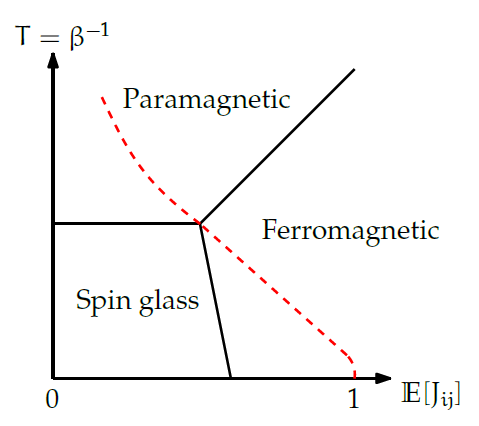
\[\mathbb{E}(\widetilde J_{ij})=\frac{e^{\beta^*}}{2cosh\beta^*}-\frac{e^{-\beta^*}}{2cosh\beta^*}=tanh\beta^*\tag{20}\]It’s a line in the phase diagram(the red dash line), known as Nishimori Line. This line don’t across Spin Glass Phase and it happens cross the tricritical point.
For the latter: Nishimori Line cross the tricritical point. We can verify it.
From (14-15), we can get the bound line between paramagnetic and ferromagnetic, between paramagnetic and spin glass:
\[para\to ferro: \beta=\frac{1}{2}log\frac{\alpha \mathbb{E}(J)+1}{\alpha\mathbb{E}(J)-1}\tag{21}\] \[para\to spin\ glass:\beta=\frac{1}{2}log\frac{\sqrt\alpha+1}{\sqrt\alpha-1}\tag{22}\]And substitute nishimori line (20) to (21):
\[\begin{aligned}\beta&=\frac{1}{2}log\frac{\alpha tanh\beta+1}{\alpha tanh\beta-1}\\e^{2\beta}&=\frac{\alpha(e^\beta-e^{-\beta})+e^\beta+e^{-\beta}}{\alpha(e^\beta-e^{-\beta})-e^\beta-e^{-\beta}}\\\alpha(e^{3\beta}-e^\beta)-e^{3\beta}-e^\beta&=\alpha(e^\beta-e^{-\beta})+e^\beta+e^{-\beta}\\\alpha(e^{3\beta}-2e^\beta+e^{-\beta})&=e^{3\beta}+2e^{\beta}+e^{-\beta}\\\alpha(e^{4\beta}-2e^{2\beta}+1)&=e^{4\beta}+2e^{2\beta}+1\\\alpha&=(\frac{e^{2\beta}+1}{e^{2\beta}-1})^2\\e^{2\beta}&=\frac{\sqrt\alpha+1}{\sqrt\alpha-1}\\\beta&=\frac{1}{2}log\frac{\sqrt\alpha+1}{\sqrt\alpha-1}\end{aligned}\]It happens equal to para to spin glass line (22). Means that these tree line intersecting at a point.
So, let the gauge model in ferromagnetic phase, we need let \(\beta^*< \beta\):
\[\begin{aligned}\frac{1}{2}log\frac{1-\epsilon}{\epsilon}&<\frac{1}{2}log\frac{\sqrt\alpha+1}{\sqrt\alpha-1}\\\epsilon&>\frac{1}{2}-\frac{1}{2\sqrt\alpha}\end{aligned}\]\(\epsilon\) is the lie probability, \(\alpha\) is the average degree(network structure). ❓Is that mean we only infer the original spin assignments when most pair lie?
Nishimori Line
Consider the model planted spin glass with Viana-Bray type. It has parameter \(\epsilon\), \(\sigma\), \(\alpha\). In the last section, two variable of Nishimori line \(\beta^*\) and \(\mathbb{E}(\widetilde J_{ij})\) at gauge model both are corrected with \(\epsilon\), the parameter of this generative model. So these two parameter normally have relationship. The inference problem with known parameter of generative model is called Bayes optimal. When we don’t know \(\epsilon\), just general \(\beta\), the line will don’t exist between \(\beta^*\) and \(\mathbb{E}(\widetilde J_{ij})\). It maybe through the spin glass phase. The Nishimori line is believed to be a general fact in inference problem with Bayes optimal setting(Known generative model’s parameter, except what we want to inference).
Factorized And Symmetric model
Generally a pairwise MRF is like (1), the joint distribution:
\[\mathbb{P}(\sigma)=\frac{1}{Z}\prod_{(i,j)\in E}\psi_{i,j}(\sigma_i, \sigma_j)\prod_{i\in N}\psi_i(\sigma_i), assume\ \sum_{\sigma_i\in\chi}\psi_i(\sigma_i)=1\]For Ising Model, \(\psi_{ij}(\sigma_i\sigma_j)=e^{J_{ij}\sigma_i\sigma_j}\), \(\psi_i(\sigma_i)=\frac{1}{2}\), \(\sigma_i, \sigma_j\in\left\{\pm1\right\}\).
For Potts Model, \(\psi_{ij}(\sigma_i\sigma_j)=\left\{\begin{matrix} e^{J_{ij}^{=}} & \sigma_i=\sigma_j\\ e^{J_{ij}^{\neq}} &\sigma_i\neq\sigma_j \end{matrix}\right.\), \(\psi_i(\sigma_i)=\frac{1}{q}\), \(\sigma_i, \sigma_j\in\left\{1,2,...,q\right\}\).
Factorized model is subclass of pairwise MRF. Symmetric model is subclass of Factorized model.
Factorized model
For \((i,j)\in E, \sigma_i\in\chi\), define(Its not the belief):
\[r^{i\to j}(\sigma_i)=\sum_{\sigma_j\in\chi}\psi_{ij}(\sigma_i,\sigma_j)\psi_j(\sigma_j)\]A factorized model defined as:
\[r^{i\to j}(\sigma_i)=r^{i\to j}, independent\ of\ \sigma_i\]This factorized definition means in a two nodes \(i,j\) model, the marginal of node \(i\): \(\mathbb{P}(\sigma_i)\) is only corresponding with \(\sigma_i\).
For explanation, we see \(r^{i\to j}(\sigma_i)\psi_i(\sigma_i)\):
\[\begin{aligned}r^{i\to j}(\sigma_i)\psi_i(\sigma_i)&=\sum_{\sigma_j\in\chi}\psi_{ij}(\sigma_i,\sigma_j)\psi_j(\sigma_j)\psi_i(\sigma_i)\\&\propto\sum_{\sigma_j\in\chi}\mathbb{P}(\sigma)_{\sigma=\left\{\sigma_i, \sigma_j\right\}}\\&=\mathbb{P}(\sigma_i)_{\sigma=\left\{\sigma_i, \sigma_j\right\}}\end{aligned}\]So if it is a factorized model, then:
\[\mathbb{P}(\sigma_i)_{\sigma=\left\{\sigma_i, \sigma_j\right\}}=r^{i\to j}\psi_i(\sigma_i)\]which is only corresponding with \(\sigma_i\).
The Ising model and Potts model both are factorized.
For Ising model:
\[r^{i\to j}(\sigma_i)=\frac{1}{2}(e^{J_{ij}\sigma_i}+e^{J_{ij}\sigma_i})=cosh(J_{ij}\sigma_i)=cosh(J_{ij})\]For Potts model:
\[r^{i\to j}(\sigma_i)=\frac{1}{q}\sum_{\sigma_i\in\left\{1,...,q\right\}}e^{J_{ij}^{=}\delta_{\sigma_,\sigma_j}+J_{ij}^{\neq}(1-\delta_{\sigma_i, \sigma_j})}=\frac{1}{q}(e^{J_{ij}^{=}}+(q-1)e^{J_{ij}^{\neq}})\]Both are independent of \(\sigma_i\).
Trivial fixed point of BP in Factorized model
The belief propagation in factorized model has a trivial fixed point(Use \(b^{i\to j}_{\sigma_i}=b^{i\to j}(\sigma_i)\)):
\[(b^{i\to j}_{\sigma_i})^*=\psi_i(\sigma_i)\tag{23}\]Substitute (23) into right side of BP (3):
\[\begin{aligned}b^{i\to j}_{\sigma_i}&=\frac{1}{Z^{i\to j}}\psi_i(\sigma_i)\prod_{k\in \partial i/j}\sum_{\sigma_k\in \chi}\psi_{ik}(\sigma_i, \sigma_k)\psi_k(\sigma_k)\\&=\frac{1}{Z^{i\to j}}\psi_i(\sigma_i)\prod_{k\in \partial i/j}r^{i\to k}\\&=\frac{\psi_i(\sigma_i)\prod_{k\in \partial i/j}r^{i\to k}}{\sum_{\sigma_i^`\in\chi}\psi_i(\sigma_i^`)\prod_{k\in \partial i/j}r^{i\to k}}\\&=\psi_i(\sigma_i)=(b^{i\to j}_{\sigma_i})^*\end{aligned}\]It’s a fixed point.
This trivial fixed point of BP doesn’t include any information in edges(the structure of network).
Stability of Trivial fixed point
The BP process can be seen as a mapping \(F:\mathbb{R}^{\mid\overrightarrow{E}\mid\times\mid\chi\mid}\to \mathbb{R}^{\mid\overrightarrow{E}\mid\times\mid\chi\mid}\). The mapped vector and mapping is \(b=(b^{i\to j}_{\sigma_i})_{(i\to j)\in \overrightarrow{E}, \sigma_i\in \chi}\in\mathbb{R}^{\mid\overrightarrow{E}\mid\times\mid\chi\mid}\), \(F(b)=(f^{i\to j}_{\sigma_i}(b))_{(i\to j)\in \overrightarrow{E}, \sigma_i\in \chi}\in \mathbb{R}^{\mid\overrightarrow{E}\mid\times\mid\chi\mid}\) where the \(f\) is the BP iteration step:
\[f^{i\to j}_{\sigma_i}(b)=\frac{1}{Z^{i\to j}}\psi_i(\sigma_i)\prod_{k\in \partial i/j}\sum_{\sigma_k\in \chi}\psi_{ik}(\sigma_i, \sigma_k)b^{k\to i}_{\sigma_k}\]Then start with \(b^0\), do the \(b^t=F(b^{t-1})\). This is the BP.
To study the stability of trivial fixed point \(b^*\), we need to get the Jacobian \(\mathcal{J}\) of \(F\).
The spectral of Jacobian matrix is a way to know the stability of fixed point. See Stability theory - Wikipedia.
Set the largest modular of eigenvalue of \(\mathcal{J}\) us \(\rho(\mathcal{J})\). If \(\rho(\mathcal{J})<1\), then the fixed point is stable, if \(\rho(\mathcal{J})>1\), then it’s unstable. If \(\rho(\mathcal{J})=1\), then it is not sure its stability.
The Jacobian \(\mathcal{J}\) is:
\[\mathcal{J}_{i\to j, k\to l}^{\sigma_i, \sigma_k}=\psi_l(\sigma_i)(\frac{\psi_{kl}(\sigma_k, \sigma_i)}{r_{l\to k}}-\frac{r_{k\to l}}{r_{l\to k}})\delta_{l, i}(1-\delta_{k, j})\]Its elements are nonzero only for directed edge pair: \(i\to j, k\to l\) satisfied \(k\to i(also\ l) \to j\), as non-backtrack path. For those edge pairs not satisfied that, the corresponding block \(\mathcal{J}_{i\to j, k\to l}\in \mathbb{R}^{\mid\chi\mid\times\mid\chi\mid}\) is 0.
TODO the derivation of \(\mathcal{J}\) is in thesis, its easy but complex.
So because of fixed point \(b^*\) has no structure information of graph, if we want BP to converge to a fixed point with structure information, then the trivial fixed point \(b^*\) should be unstable. As:
\[\rho(\mathcal{J}|_{b^*})>1\]is a necessary condition for BP to converge to informative marginal.